For BI and analytics projects to be successful and transform the way people manage their decisions, speed is often a necessity. It’s not enough to have the right KPIs or the ability to consume those easily; the capacity to Get Insights Faster™ over taking a coffee break every time a dashboard is loaded or a new business question is asked is imperative for success.
The endgame – Fast analytics
For pre-defined content such as dashboards or reports, a proper data retrieval design that speeds up the load time will not only ensure a smoother experience for consumers but will also minimize the load on the data source (for example, a database server). Less load on the database server often means other purposes are served faster, which ultimately results in happier users and less concerned database administrators!
Where ad-hoc data discovery is concerned, users may start with a simple query that retrieves data quickly, but as they dive deeper into the data and add additional fields and calculations, and join additional tables, etc., they may find that the query performance has slowed as the query increases in complexity.
In both cases, using In-Memory data storage is often the recommended alternative to enable a faster and better solution, however, it is not always the right option, and other factors should be taken into consideration as well. This post will focus on Dundas BI’s In-Memory Engine and the role it plays in optimizing performance.
So let’s dive into it!
Dundas BI storage types for performance optimization
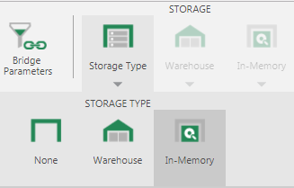
Dundas BI allows you to optimize performance by taking advantage of different storage types available in the data cube layer, which is Dundas BI’s optional data preparation layer. The different storage types are as follows:
- By default, the storage type is set to None, meaning that data retrieval occurs in real-time. For example, when a user loads a visual, a query will execute in real-time against the data source and the latest results will be sent back to the user.
- The Warehouse storage type lets you store the results of your data cube model in Dundas BI’s Warehouse database, which is a relational database. For example, if a data cube is configured to query data from both an Excel file and an Oracle database and then join the results, it may take more than a few seconds if done in real-time. If the Warehouse storage is used, Dundas BI will perform the queries when the data cube is built (typically on a schedule, i.e., every 15 minutes) and then store the results of the queries join, so when a user loads a visual, Dundas BI will query the Dundas Warehouse database instead of the data sources. Querying the results of the join (or any other data transformations) is typically faster than querying raw data and waiting for the join to be done, thus delivering a performance gain.
- The In-Memory storage type operates similarly to the Warehouse storage type, but instead of storing the results on disk within Dundas BI’s Warehouse database, it stores the data in Dundas BI’s server memory (RAM) using a proprietary structure for even greater performance gain potential.
Once the data cube has been designed, that model can be kept in one of the storage options by selecting the option from the menu available from the data cube designer toolbar.
Both storage types can be built either on-demand or scheduled to run periodically. Scheduling is particularly useful when a line of business database is either not permitted to be queried during specific time periods e.g., during the day, or real-time querying of data is not needed. In this case, schedule a storage operation to run at a particular time (i.e., run a nightly build so that during the day, data retrieval queries are made against the Warehouse or In-Memory storage only).
Note that on a single dashboard (even on a single visual) it’s possible to combine data coming from all of the different storage types, so for example, it’s possible to have a dashboard with data stored In-Memory next to data extracted in real time from your data sources.
Finally, it is important to mention that regardless of the selected storage type, by default, Dundas BI will always store the visual’s data results for 20 minutes. For example, regardless of the storage type, if a user loads a certain dashboard and the same dashboard is loaded with the same filter values within 20 minutes, the data results for the dashboard visuals will be extracted from the server cache memory. This is opposed to going back and querying the data sources or the Dundas BI storage again. The default time for saving cached results can be changed by setting the Result Cache Absolute Expiration under the application configurations or can be by-passed at the individual metric set level. This particular results cache shouldn’t be confused with Dundas BI’s In-Memory storage, although they both use the server RAM.
Deep dive into the In-Memory engine
What is it?
The In-Memory storage type stores the data result from the data cube in Dundas BI’s server memory. The In-Memory cube data is also persisted to Dundas BI’s Warehouse database so that it can be reloaded back into memory in the event of a server restart.
The In-Memory analytical engine uses hypergraph structures for organizing data extracted from the data sources. A hypergraph is a mathematical concept and is a generalization of a graph in which an edge can join any number of vertices. Hypergraph’s do not store all possible coordinates. Dundas BI’s In-Memory engine utilizes a proprietary (patent pending)* algorithm that implements this concept. For example, data aggregations across multiple hierarchy levels are pre-calculated and stored in a tree-like structure in the available RAM.
In such a system, performance and memory usage are critical. Performance relates both to the time required to build the hypergraph representation (store the data result In-Memory) and the speed of data retrieval (querying).
*Update - Dundas was awarded a patent for its In-Memory Engine; technology that optimizes the performance of data analysis by computer.
When to use it?
The decision to use a storage option, whether Warehouse or In-Memory, is dependent on a few factors. One major factor is when the data source is slow to execute the queries or when data cubes are built with many transformations that are slowing the overall data retrieval. Alternatively, even if the data retrieval is not fast, it’s not ideal to load the data source with too many queries as that will slow it down, especially if that data source is used by any other line of business.
The decision to use In-Memory vs. Warehouse storage depends on a variety of factors related to data and the resources available. In general, In-Memory processing is faster than Warehouse due to the optimization process it utilizes. In-Memory uses memory to store the model’s results and fetching data from memory is faster than querying it from the disk. The caveat is that In-Memory is more expensive to use because of higher memory utilization, which typically, is not as readily available as disk space. If memory is available on the server or if investment in additional memory is not an issue, then In-Memory is preferred as it is faster than Warehouse. That being said, in many cases the difference in retrieval time between data stored in the Warehouse vs. the memory isn’t noticeable, hence it’s recommended to start with the Warehouse and check the performance of the query with it. If the performance is satisfactory, continue using this option and avoid unnecessary usage of RAM memory. If the performance does not meet expectations, then opt for In-Memory storage.
How to set up?
Setting up and storing data In-Memory is a simple process. Once the data cube has been designed, open the data cube designer toolbar and set the Storage Type to In-Memory.
Once the In-Memory storage type has been chosen, check the data cube to make the In-Memory settings available. After checking in, a Start In-Memory Processing prompt will appear. Click OK to begin building In-Memory storage, or click Cancel to build it later as shown below.
Alternatively, the In-Memory model can be built on the fly can be scheduled to run periodically and get refreshed results for specific time periods.
For detailed setup, please refer to this article: Data Cube storage types
Advanced Settings
To maintain a stable usage of the RAM, the In-Memory storage compresses and decompresses the data cube results as required to free up memory resources. The recompression can be prevented by disabling the memory management from the Configure Data Cube option on the toolbar. Using this option, the data cube results will always be in a decompressed state, meaning any queries made against it will be faster by skipping decompression steps, thus increasing the data retrieval speed.
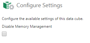
However, using this option will cause the results of the data cube to continue to expand and consume as much memory as it requires, which may cause the system to run out of memory and lead to memory paging. This may lower the performance rather than improve it. Therefore, it’s recommended to use this option only for the data cubes that are the most important and which require the fastest queries.
For more information on this option, please see:
At the application level, the In-Memory engine can be further customized to suit the environment via several advanced settings. Those are available under the Data In-Memory Cube Engine category within the application configurations (Admin -> Setup -> Config):
Cache Cleanup Threshold
This setting is used to set the threshold of utilized memory on the server before the In-Memory engine begins a cleanup process to free up more space. The cleanup process will actually compress more of the data cube result’s stored In-Memory, meaning it’s consuming less memory on the server. The threshold is defined using a percentage. For example, if it’s set to 50% and the server has a total 16GB of RAM, the engine will start the cleanup when 8GB of the server RAM has been utilized.
Cache Polling Interval
This is the polling interval in milliseconds that is used to check for the Cache Cleanup Threshold. For example, by setting the interval to 500, every half-a-second the system will check if the cleanup threshold has been reached. The cleanup process will begin if the threshold has been reached.
CPU Cores
This is the total number of CPU cores dedicated to the In-Memory storage processing. For example, when set to 4, only four cores of the server will be utilized for the process. The default value is 0, meaning the application will use all available CPU cores. This setting is useful when limiting the number of cores to be used for the process.
Load Wait Time
The data cube result that is being stored In-Memory also gets stored in the Warehouse database to keep a copy in case the server memory is wiped (for example, when the server restarts). This allows the data cube result to be re-used without having to re-build the cube. The Load Wait Time is the maximum wait time for the data to load from the Warehouse to the memory. If the load takes longer than this time, a timeout error will appear.
Memory utilization when using in-memory storage
One of the common questions that arise when using In-Memory storage is regarding the resources required and consumed and the time it takes to build one. Note the minimum RAM recommended for using In-Memory storage is 16 GB and depending on the usage, often times, the available RAM is increased to boost performance. It’s not uncommon to have servers with 32 or 64GB of RAM when In-Memory storage is heavily used.
Dundas BI is a .NET web application running on an IIS web server meaning the overall memory of the application is managed by the .NET process, which handles other items aside for In-Memory data cube results. This together with some factors such as the hardware specs of the server, the number and complexity of the data transformations within the data cube, and the nature (size and structure) of the data cube results, define the memory utilization and the build speed of the model.
The size of the data cube result is, of course, an important factor, but more importantly, it is the number of hierarchies and unique hierarchy members (cardinality) that are being used in your data cube (see the data cube process results). As the data cube result tree structure grows larger, increasing the number of hierarchies or member hierarchies can exponentially increase the memory usage. As a best practice, to minimize memory usage and processing time, it is recommended to only keep necessary hierarchies within the data cubes stored In-Memory. From Version 6 onwards, attribute hierarchies can be utilized in order to reduce the number of hierarchies to be processed. Attribute hierarchies contain other hierarchies that provide details about or describe a particular hierarchy. E.g., Products can be described by their Color, Size, Class etc. and can be selected as Attribute Hierarchies for the Product hierarchy. In the data cube, four hierarchies are reduced to one hierarchy. This reduces the number of hierarchies to be processed in-memory significantly thereby reducing the memory usage. The advantage of this approach is that the attributes automatically become available when using the hierarchy in a metric set and can be displayed on a visual. More information on how to use attribute hierarchies in the data cube can be found here. It is also recommended to separate data cubes that relate to different business domains, each with unique sets of measures and hierarchies. For example, two separate data cubes should be created for HR and Marketing data, as both domains are highly unlikely to share the same measures between them.
Optimizing the In-Memory builds is also achieved by minimizing the number of measures, and the supported aggregators for each, in the data cube process results (for example, remove average supported aggregation for measures that should never be averaged, etc.). Similar to the number of hierarchies, reducing those options will limit the size of the In-Memory tree structure built, yielding a faster build time, smaller memory consumption and faster data retrieval.
Since many different factors determine the memory utilization, the answer to how much time and RAM is required to build data cube results into memory can vary greatly and is difficult to estimate. Generally, if the In-Memory storage result fits entirely into the available RAM, then on a typical 8 core server, the total build time will generally be divided equally between retrieving/loading data from your data sources and building the In-Memory storage. A good starting point for estimation is to look at the query time of the data from the source. Note that increasing the number of processing cores will reduce the time to build the In-Memory data structures thanks to parallelization.
Use case example
An example of the performance optimization achieved using the In-Memory engine can be seen in the Big Data Analytics dashboard sample available in our samples gallery. The sample connects to a Google BigQuery database containing a total of 137,826,763 rows.
Experimenting with the interactions of this sample (by clicking on the different data points), shows the load times are instantaneous. When executing queries in real-time against Google BigQuery (i.e., no data storage is used for some visuals), simple queries of one measure and one dimension return the result in approximately 5 seconds. This is quite impressive for this volume of data, but it can be optimized even further when executed against an In-Memory stored data cube in Dundas BI, which returns the data instantaneously as demonstrated in the sample.
This is not to say that the default should always be to use In-Memory storage. In a real-world example, there are typically combinations of the different storage types to optimize the user experience as well as to best utilize the available server resources (RAM and disk space). Many data sources such as Google BigQuery and other big data analytical databases (Amazon Redshift, HPE Vertica, Exasol and others) are capable of producing query results very quickly where using pre-defined storage isn’t needed, meaning using no storage is the optimal way to go.
Hopefully, the above information will help when it comes to choosing the optimal way to manage data within Dundas BI.
Follow Us
Support