Cohort Analysis enables you to easily compare how different groups or cohorts of people (i.e., customers) behave over time. It gives you visibility into the life-cycle pattern of different groups so you can draw insight regarding items such as customer retention trends and the health of your business processes over time.
For example, you can compare customers you’ve acquired in the past year with those acquired several years ago, or compare users who’ve joined over the holiday season with another group that joined in the summer, and see if those holiday shoppers stuck around.
What is a Cohort?
Before getting into the nitty gritty details of cohort analysis, let’s take a moment to define the term “cohort”. A cohort is a group of people who share a common characteristic over a specified period. For example, a group of students from a university who graduated in 2011 is a cohort. All of the students in this cohort graduated in the same year, and this is their commonality.
Cohort analysis is the study that focuses on the activities of a particular cohort. If you calculate the average income of these students over the course of a five year period following their graduation, you would be conducting a cohort analysis. It allows you to identify relationships between the characteristics of a population and that population's behavior.
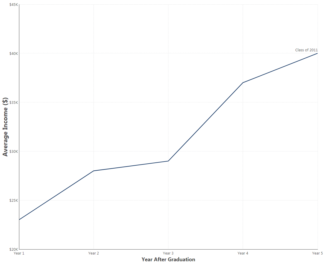
Figure 1: You can see a trend of how the Average Income for this graduating class increases over the years
Keeping with the graduating students’ example, you can examine another graduating class, say, 2012, and compare their five-year average income to that of the class of 2011. When looking at the average income over the five years post-graduation in comparison to the income of the 2012 students over the same relative interval, you’ll get a unique apples-to-apples comparison of these groups. In this case, there appears to be a relationship between a student's year of graduation and their income.
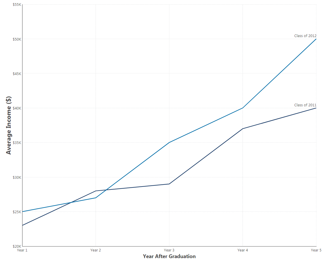
Figure 2: Here, we can see that both graduating classes increase their average income per year. However, by the third year out, the 2012 grads make more on average than their 2011 counterparts (by an increasing margin).
This is just one of the many use cases of Cohort Analysis. By analyzing the different cohorts in your data, you can also:
- Examine where cash flow is coming from and understand the health of your business
- Easily see how much monthly or quarterly revenue is driven from newer and older cohorts
- Study customer retention patterns to see if they are getting better or worse (for example, as a result of a change in your customer service)
- Compare cohorts of users from different segments to find the most and least valuable segments
In this blog, we will focus on such a use case and discuss how to implement it in Dundas BI.
Cohort Analysis Using Dundas BI
Let’s say you want to better focus your marketing campaigns. To do so, you want to analyze which customers provide you with the most repeat business and when they do so based on the time of the year (month) they became a customer. One of the ways to analyze this, is by using the Period-over-period analytics capability. However, this will only give you the total revenue generated over the year in comparison to the previous year. If you want to know which specific groups of customers contributed to that revenue, you’ll need to group them into cohorts.
Cohorts can be formed depending on the month your customers first purchased from you.
To perform the cohort analysis, a typical dataset should include one record per customer purchase. Each record contains a customer's ID, the date and time of the purchase, the amount of the purchase, and the customer's "cohort date" (in this example it would be the date (month) of the customer's first purchase).
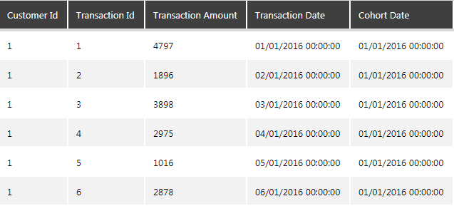
Figure 3: Typical dataset to perform cohort analysis
The tricky part here is to get the cohort date, which can be accomplished as part of your data retrieval (i.e., using a sophisticated SQL query) or by calculating the cohort date in Dundas BI using the built-in data preparation layer (“Data Cube”) as shown in the steps below.
Preparing the data
For this example, we are going to use a sample dataset that tracks the retail transactions per customer and segment customers based on their first date of purchase to track the cumulative spending for each cohort.
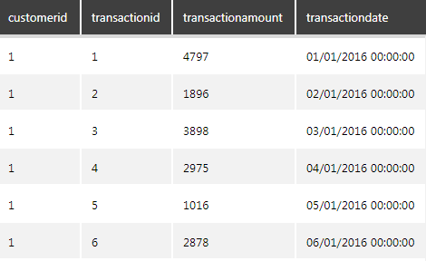
Figure 4: Retail transactions dataset
Step 1: Calculate the Cohort Date
To calculate the cohort date, we need to identify each customer’s first date of purchase. The easiest way to do this is by taking the minimum transaction date and grouping by customer (you can then rename the transaction date to cohort date). Then we will take this dataset and join it with the same transactions table using the customerid. To do this, drop the transactions table twice on the data cube canvas and configure one of the SQL Select nodes to apply the MIN function on the transaction date and group by the customerid by editing both the columns as shown below.
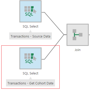
Figure 5: Configure the SQL node to calculate the Cohort Date
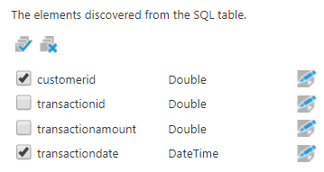
Figure 6: Select the customerid and transactiondate columns
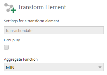
Figure 7: Apply the MIN function to the transactiondate column
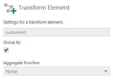
Figure 8: Group by the customerid column
Next, join the two SQL nodes in the customerid column using the Join transform.
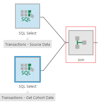
Figure 9: Add a Join transform to join the two SQL nodes
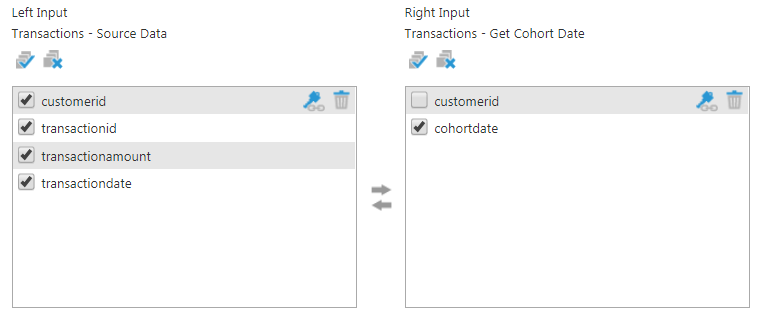
Figure 10: Join on the customerid column
The result will look like this:
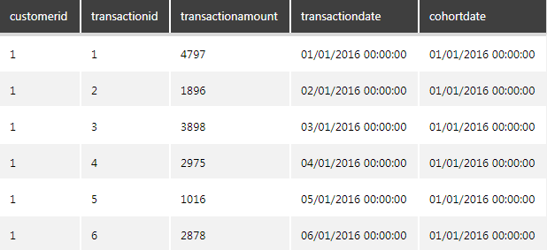
Figure 11: Result of the join
Step 2: Create Cohort Identifiers
Now that we’ve calculated the cohort date, we can segment customers into cohorts based on the month in which they made their initial purchase. To do this, we first need to translate each cohort date value into a meaningful name that represents the cohort – in this case, it’s the year and month of their first purchase. To get these cohort names, we’ll use a Calculated Element transform to extract the Year and Month from the Cohort Date column and combine them into one column as shown below.
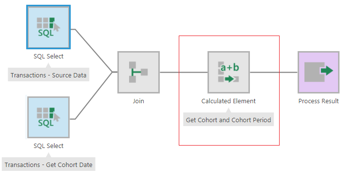
Figure 12: Add a Calculated Element Transform to get the Cohort and Cohort Period
Configure the Calculated Element transform and add a calculated column called “Cohort” of string data type and use the script below to return the cohort.
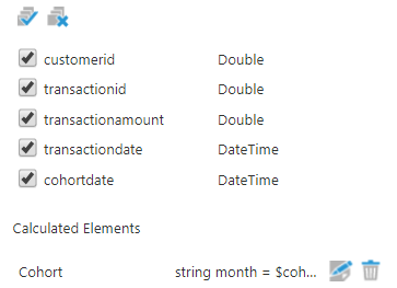
Figure 13: Add a column to calculate the cohort
string month = $cohortdate$.Month.ToString();
string year = $cohortdate$.Year.ToString();
string MonthName;
if(month == "1")
MonthName = "Jan";
else if(month == "2")
MonthName = "Feb";
else if(month == "3")
MonthName = "Mar";
else if(month == "4")
MonthName = "Apr";
else if(month == "5")
MonthName = "May";
else if(month == "6")
MonthName = "Jun";
else if(month == "7")
MonthName = "Jul";
else if(month == "8")
MonthName = "Aug";
else if(month == "9")
MonthName = "Sep";
else if(month == "10")
MonthName = "Oct";
else if(month == "11")
MonthName = "Nov";
else if(month == "12")
MonthName = "Dec";
return String.Concat(MonthName, " ", year);
This column will be the “Cohort” that we will use to segment the data.
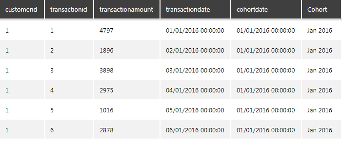
Figure 14: Result of the cohort calculation
Step 3: Calculate Life-cycle Stages
Once the cohorts have been identified, the next step is to determine the “Lifecycle stage” that shows when each event, in this case, each transaction, happened for that customer after their first date of purchase.
For example, if a customer made their first purchase on January 10th, 2016, and their second purchase on March 15th, 2016, they would be in the "Jan 2016" cohort. Their first purchase would be in the "Month 1" lifecycle stage (that is of course always the case), and their second purchase would be in their "Month 3" lifecycle stage because it happened in their third month after becoming a customer.
To calculate the lifecycle stage for a particular transaction, we'll need to determine the amount of time between the customer's first purchase and the purchase in question. This can be done using the same Calculated Element transform as used to calculate the cohorts. Add another calculated column called “Cohort Period” of string data type and use the following script that calculates the difference between the cohort date and transaction date in Months:
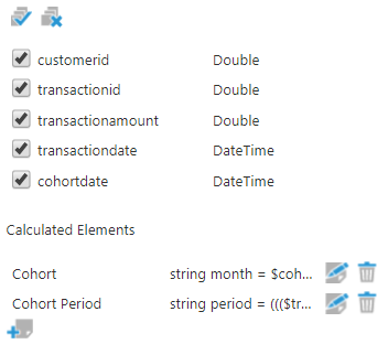
Figure 15: Add a column to calculate the Cohort Period
int period = ((($datetime$.Month -$CohortDate$.Month) + 12 * ($datetime$.Year - $CohortDate$.Year)))+1;
return String.Concat("Month ",period.ToString());
Rename the columns to make the names user-friendly and the final result will look like this:
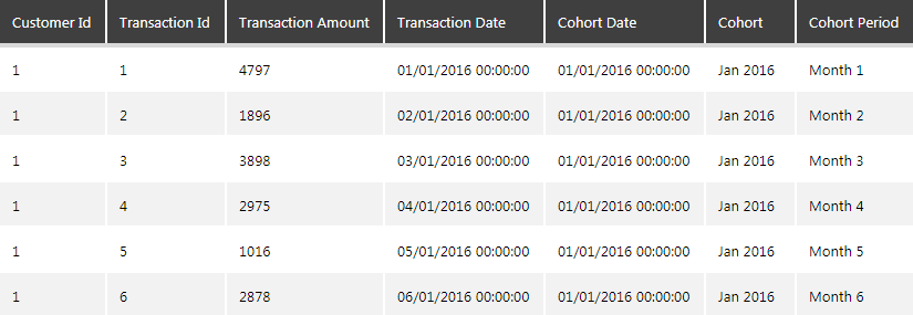
Figure 16: Result of the Cohort Period Calculation
Visualize the data for analysis
Once you have the data ready, you can now analyze it in a visual form. Create a metric set, and from the data cube created, add the Transaction Amount as a Measure, Cohort Period as a Row and the Cohort as a Column (series).
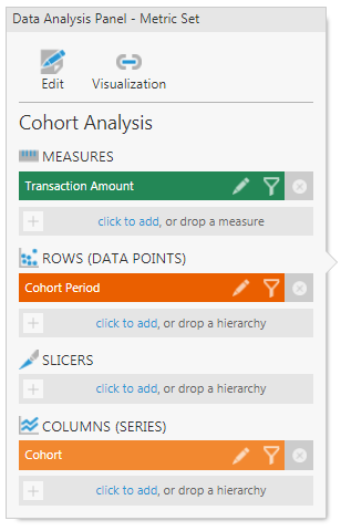
Figure 17: Data Analysis Panel on a Metric Set
To get the cumulative total, add a CMLTOTAL formula on the transaction amount column.

Figure 18: Calculate the Cumulative Total
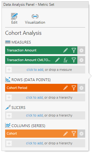
Figure 19: Cumulative Total column gets added as a Measure on the Data Analysis Panel
Re-visualize as a line or a curved line chart to see the trend (you can hide the transaction amount series from the chart properties to just focus on the cumulative total).
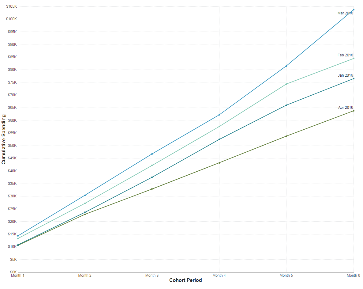
Figure 20: Cumulative spending of each Cohort over the course of 6 Months
Conclusion
The chart created is a cohort analysis that views each cohort's spending as a cumulative value over time. This allows you to watch total customer lifetime spending growth, over time per cohort.
For example, based on this trend, you can deduce that the customers who made their first purchase in April 2016 tended to spend far less over the course of the next six months whereas the customers who made their first purchase in March 2016 tended to spend the most over the course of the next six months. More specifically, you can identify that marketing activities such as campaigns and promotions that occurred at the beginning of the year (from January to March) helped to increase repeat business activity. You can also identify that something changed in April that caused a significant drop in the likelihood of those customers returning for more business. If you are looking at this data as a marketer, this provides valuable insight into the customer purchase behavior and can help to plan targeted campaigns and user experiences based on the performance of the cohorts.
The above is one such example of cohort analysis. You can also segment it further by including in your dataset additional attributes such as the customer's referral source, the first product they purchased, geographic and demographic information, etc. The data can also be normalized by the size of the cohort. To do this, each data point for a cohort must be divided by the number of members in that cohort. That way, you can view the average value per cohort member side-by-side without bias from the size of the cohort.
What’s important to glean from this blog, is that Cohort Analysis can enable you to effectively compare behavioral trends of different groups over time. It can allow you to ask very specific questions (such as we’ve done above, and others pertaining to retention trends and business process health, etc.), analyze only the data that is relevant to that question, and take action on the insights you’ve uncovered. What’s more, is that this advanced analytics functionality can be easily performed within Dundas BI.
Here are some other blogs we think you’d be interested in:
Follow Us
Support