Using a data cube to join tables

Contents[Hide]

1. Overview

Use data cubes to integrate data from different sources, transform the data, and produce a reusable data model with optional data storage capabilities.

This walkthrough shows you how to:

Create a new data cube.
Set up an ETL process consisting of transforms.
Use transforms to join three database tables.
Link the output columns of a data cube to existing hierarchies.

You need to be a user with a Developer seat to create or edit a data cube. The figures use the Adventure Works for SQL Server 2012 database as an example.

Related video: Introduction to Data Cubes

Tip

When editing a metric set, you can also join tables and data sources automatically without editing a data cube.

2. Walkthrough

2.1. Create a new data cube

From the main menu, click Data and then Create. Choose the Blank option to drag and drop data sources as in this example.

Otherwise, you could choose to start with one of the listed input transforms, or add one of them later from the toolbar.

Note

You need to be a developer user to create and edit data cubes.

The data cube editor is displayed.

2.2. Add a database table

Next, locate your existing data connector in the Explore window and expand it to list its available data structures such as tables. We will drag the [Sales].[SalesOrderDetail] table to the canvas.

When you add the first data source, Dundas BI automatically creates a simple ETL process consisting of two transforms, with data flowing from left to right. A data cube name is automatically assigned and displayed in the status bar at the bottom, which you can double-click to rename.

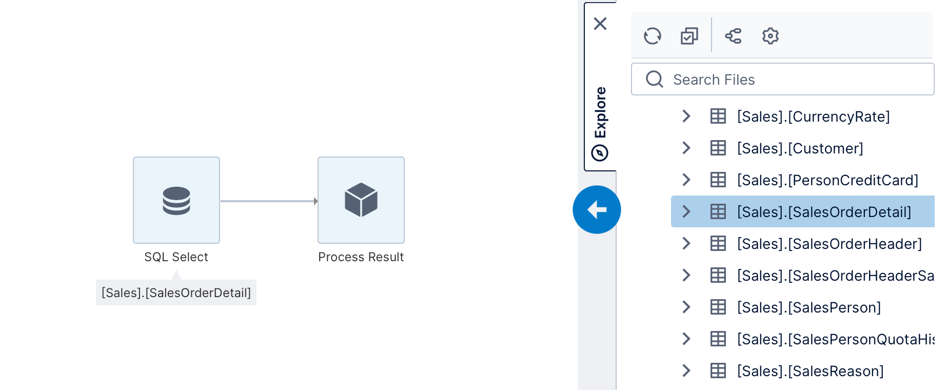
The first node in the ETL process is a SQL Select transform, which represents a query to select data from the [Sales].[SalesOrderDetail] table.

The second node is a Process Result transform, which represents the output or result of the data cube (ETL process). This transform doesn't do any data processing but allows you to configure the way the data is made available to users accessing data from the cube.

An ETL process can have multiple inputs (for example, multiple Select transforms that query data from different databases) but always only a single output (the process result).

2.3. Add a second database table

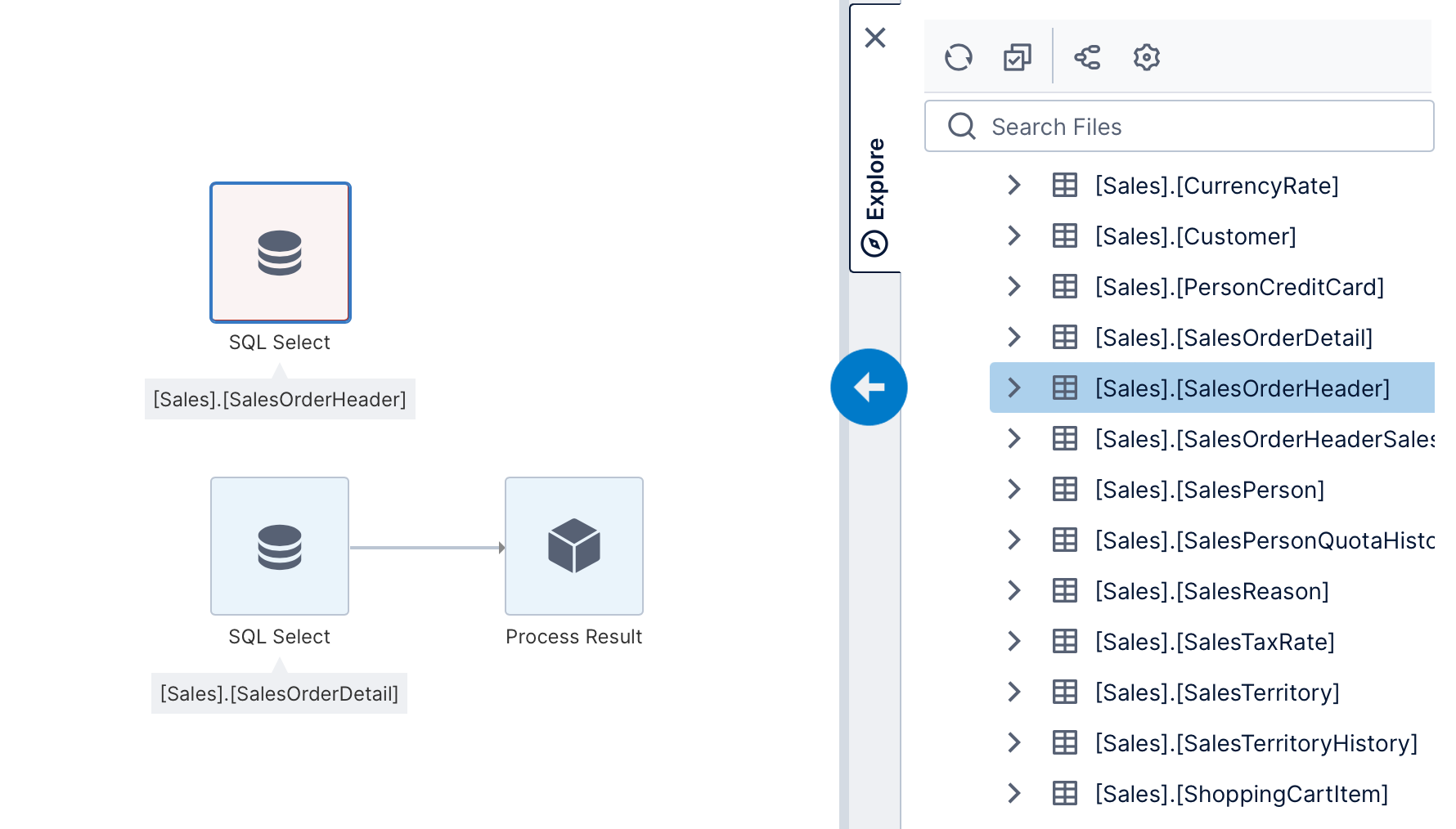
Add the second table [Sales].[SalesOrderHeader] to the canvas. The second SQL Select transform is displayed in red because it is not yet connected to the ETL process.

2.4. Insert a join transform node

To insert a transform directly in a specific place, click to select a connection link such as the one connecting our first SQL Select transform and the Process Result transform.

From the toolbar, click Insert Common and select Join for this example. In other scenarios, you may want to use other transforms such as Union or Fusing to combine data together.

Select connection link and insert Join a transform

Note

Most transformations are incorporated into a query to be executed by your database or other data source in order to optimize performance. Certain transforms such as Calculated Element can introduce icons with an exclamation mark in the top-left corner of the transform, indicating that data will be taken in-memory for processing at this point.

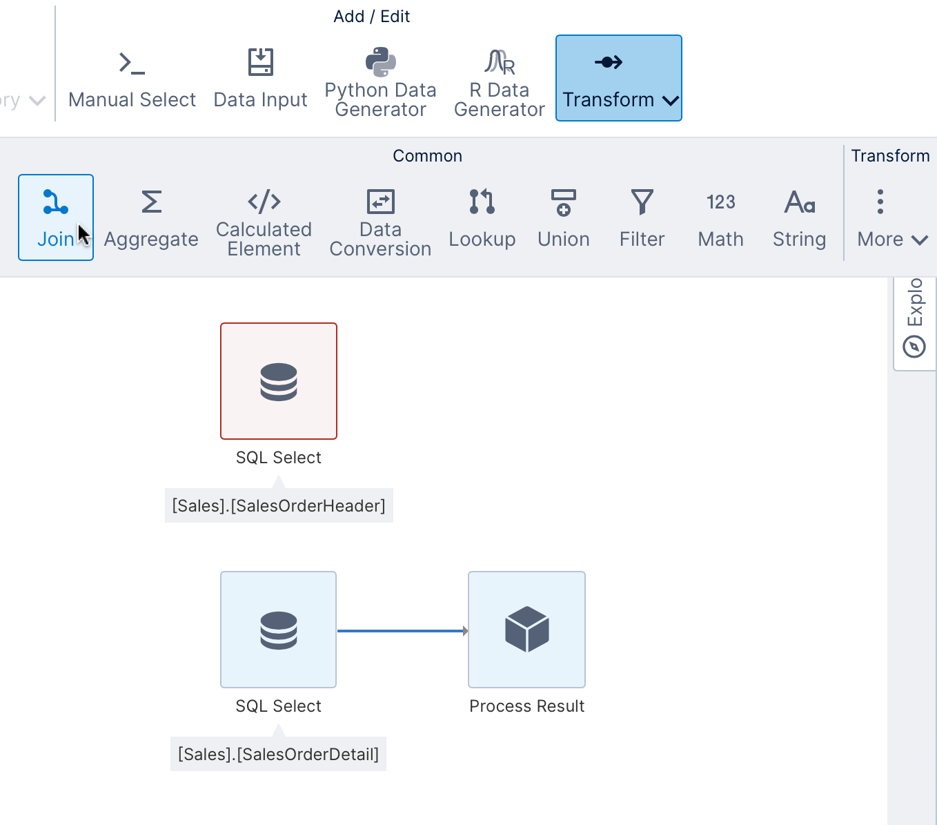
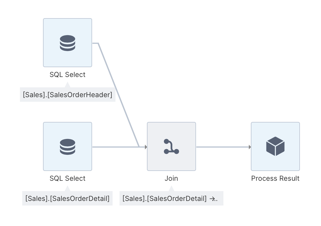
A Join transform is inserted into the ETL process where a connecting link was selected as shown next. If a connecting link was not selected, click and drag from another transform to the new transform to draw a connection between them.

The join transform needs two inputs, and is displayed in red until it has both required inputs connected.

2.5. Connect the 2nd select transform to the join transform

Click and drag a connection from the 2nd input to the join transform.

Tip

If you make a mistake connecting transforms, you can break a connection link by clicking the link and choosing Disconnect from the toolbar or from its right-click context menu.

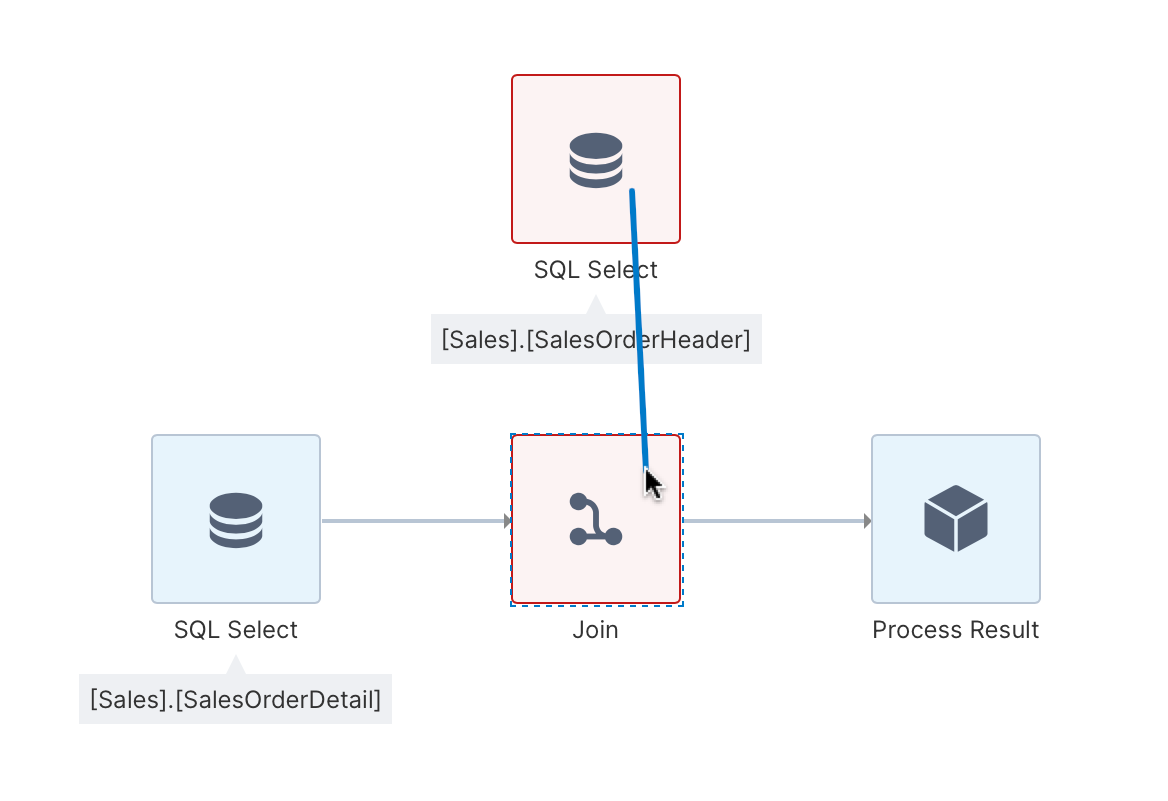
Alternatively, you can hold the Ctrl or Shift keys while clicking to select the two transforms, and then choose Connect in the toolbar.

With both SQL Select transforms connected to the join transform as inputs, none of the transforms now appear in red.

Tip

As a shortcut, you can simply drag a connecting line between the two transforms that you want to join instead of adding and connecting the join transform yourself, as shown later.

2.6. Configure the join transform

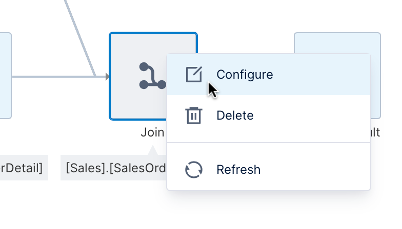
Once the join transform has been connected, you typically need to configure it. To configure any transform, select it and choose Configure in the toolbar or from its right-click context menu.

The Join configuration dialog is displayed.

Hovering over a key binding in the join configuration dialog

Tip

Hover over one of the columns with a key icon to highlight its match in the other list as shown above.

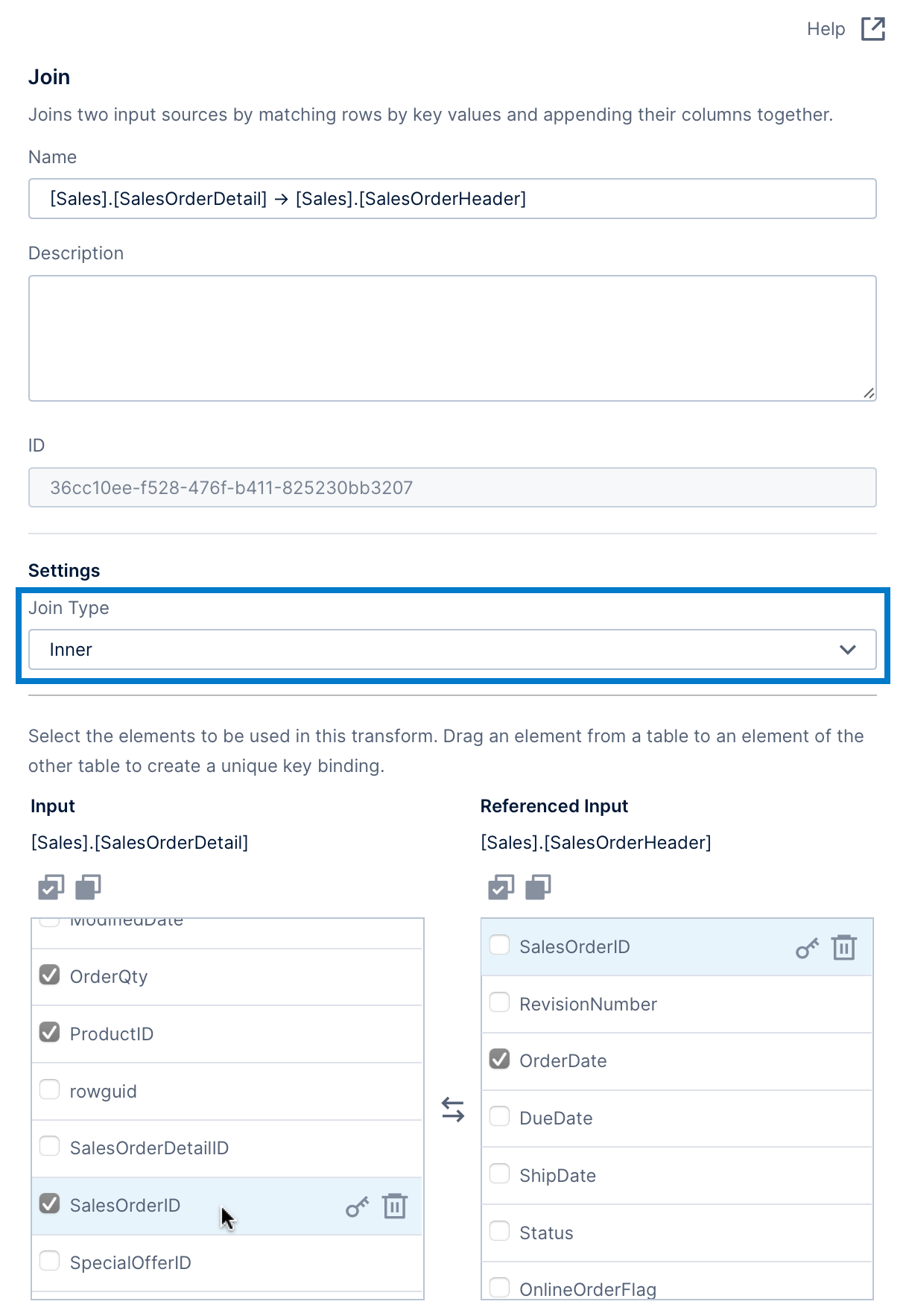
There are three main ways to configure a join:

Choose the Join Type (which can be Inner, Left, Right, or Full). This examples uses Inner because it assumes matching IDs exist in both tables.
Set up the unique key binding, which will be indicated by key icons next to columns containing matching values from each table. There may already be one added automatically like for SalesOrderID in our example based on relationships already defined in the database or by a user in Dundas BI. Otherwise, drag a column from one list and drop it over the matching column from the other list as shown later.
Use the checkboxes to select or de-select columns for inclusion in the output. For example, select OrderQty, ProductID, and SalesOrderID from the order details, and OrderDate and SalesPersonID from the order headers.

See the Join transform article for more details on these options.

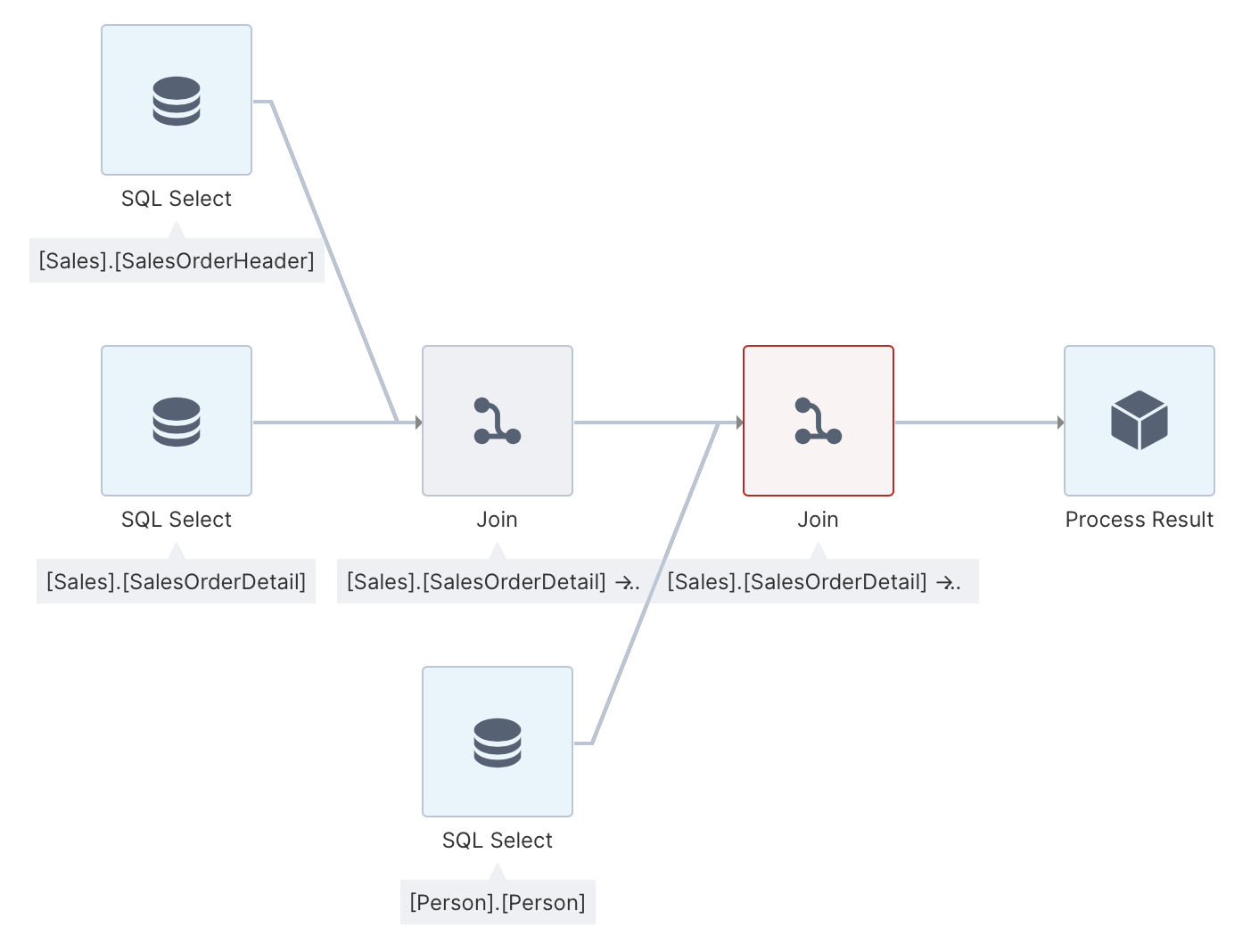
2.7. Join with a third database table

The ETL process so far joins two database tables. To add a third table, you will need to insert another join transform into the ETL process because each join accepts only two inputs.

In the Explore window, locate the [Person].[Person] table and drag it to the canvas. The table appears as a third SQL Select transform, displayed in red because it is not connected to the ETL process yet.

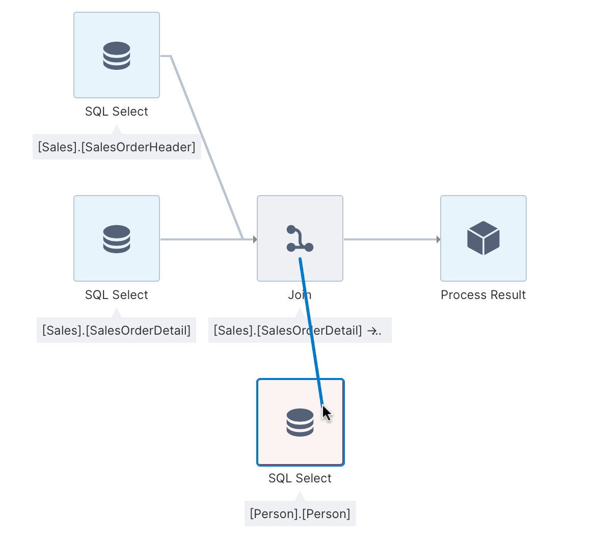
Click and drag a connection between two inputs to join them together as a shortcut

You can insert a join transform and then click and drag to connect its inputs like in the first example, or as a shortcut simply click and drag a connection from one transform that you want to join to the other to automatically insert and connect a join transform.

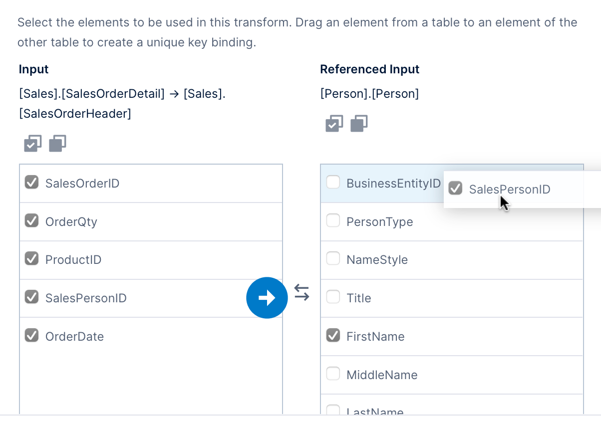
2.8. Configure the 2nd join transform

Once the second join transform is connected in this example, it must be configured. Select it and choose Configure from the toolbar or context menu.

For this example:

Choose Inner as the Join Type.
Add the unique key binding by dragging the SalesPersonID column from the sales order data and dropping it onto the BusinessEntityID column from the Person table, which in our example contains matching key values.
Finally, de-select all column checkboxes from the Person table except for FirstName to exclude the others from the output.

Dragging SalesPersonID onto the matching column on the right

2.9. Configure the process result

The last step of the ETL process is the Process Result, where you can configure the final output of the data that users with read access will see when using it as a data source in metric sets.

Click the Process Result transform to open the Data Cube Elements panel, which shows the list of measures (numeric) and hierarchies (usually non-numeric) output from this data cube. Click on an element or its pencil icon to edit its settings.

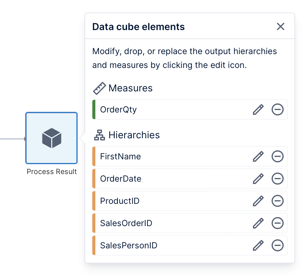
You can customize each element's name, description, predefined formatting, and more.

Any data not used as a measure becomes a hierarchy when output from the cube whether or not it was based on a hierarchy you defined ahead of time to contain multiple levels or other customizations. If not replaced with a predefined hierarchy, a column of data becomes an 'implicit' hierarchy.

To replace an implicit hierarchy with your own that's based on matching key data, click Select a hierarchy or level to use as a replacement. In the Open dialog that appears, select the hierarchy, or expand it and select a particular level that matches the column's values. Click the Open button at the bottom to proceed.

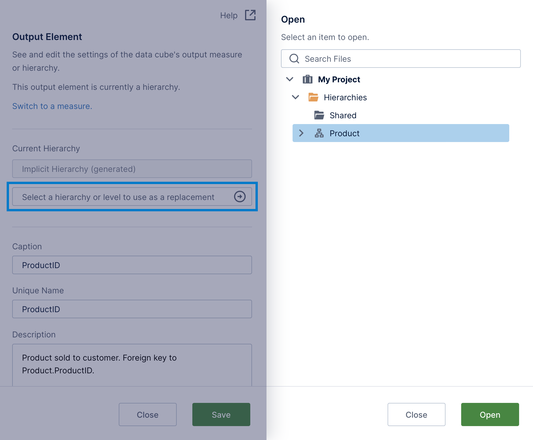
Selecting a hierarchy to use as a replacement

The steps are the same to replace a DateTime type column (such as OrderDate in this article's example) with a hierarchy from the built-in time dimension or from one of your own, to group by and drill down between levels such as Year and Month.

For more details on these options, see the Process Result article.

2.10. Data preview

Open the Data Preview window to preview the data processed up to whichever transform is selected. With Process Result selected, this shows the data as output by the ETL process (before replacing the raw data with hierarchies).

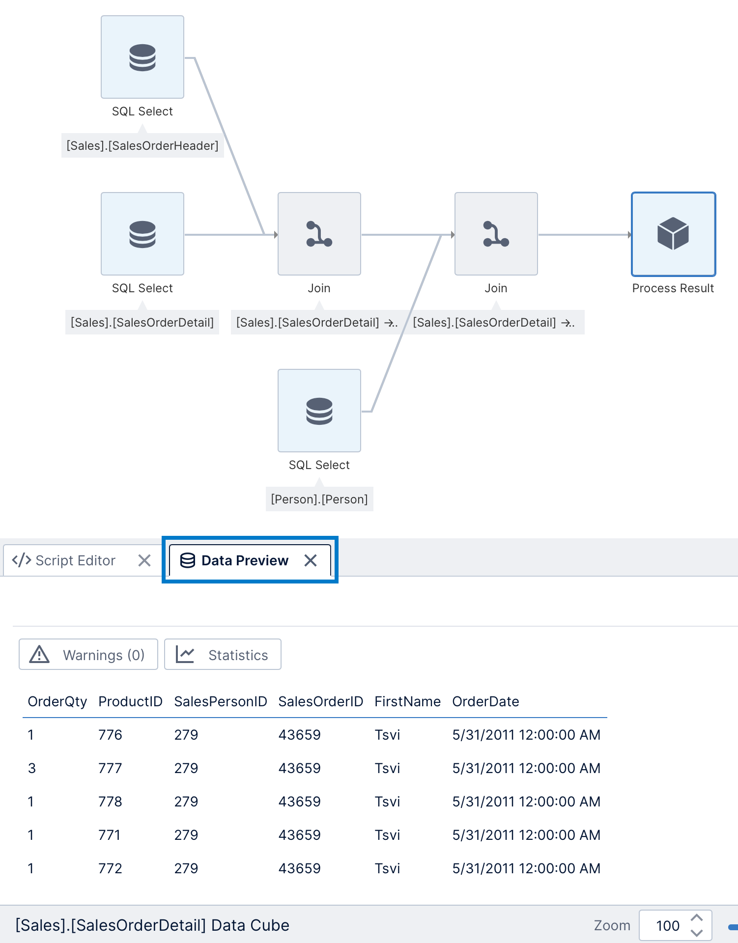
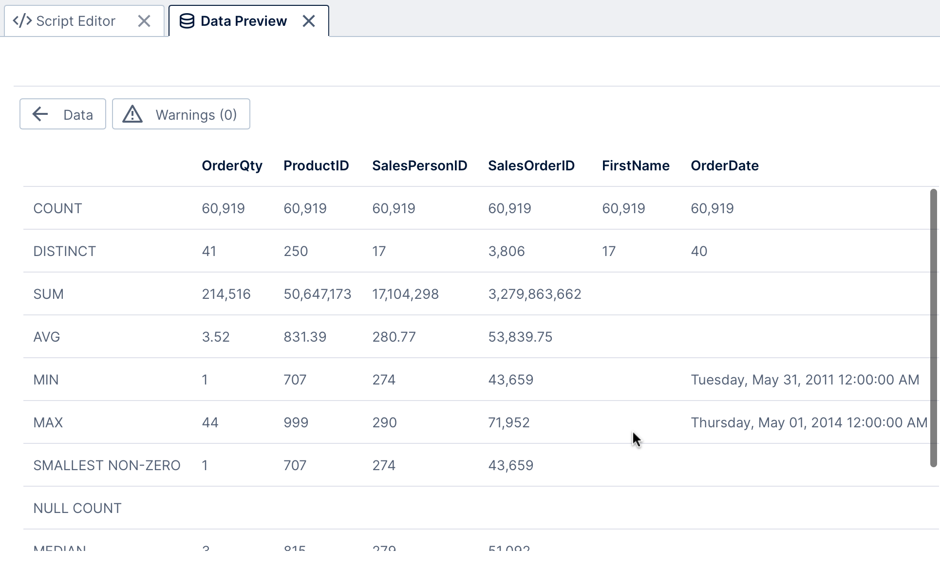
Click Data Preview to preview the resulting data

The row above the table provides access to warnings and statistics about the data.

Click Statistics to view a summary of each column, such as the average, minimum & maximum, distinct count, and the number of null values (which can result in Unknown members when used in metric sets).

2.11. Check in

Check in your data cube from the toolbar so others can use it too. Everyone with access to the cube with a power user seat or higher can use its data to create metric sets.

2.12. Reusing in other data cubes

You can reuse the process flow of a data cube in other data cubes to avoid setting up the same transforms multiple times, simply by dragging another data cube onto your canvas.

For details, see the Data Cube transform.

Welcome to Dundas BI Support