
Exponential Smoothing
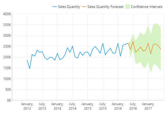
The Forecasting and Exponential Smoothing functions use exponential smoothing models to predict future values based on an analysis of historical time series data. These models apply an exponentially-decreasing weight to historical data in order to forecast future values based on emerging trends and can consider seasonal effects.
These functions are typically used with a date/time axis but will also work with a numeric hierarchy or measure as the first input. Also look for the Forecast Analysis option recommended in the Re-Visualize menu to apply these functions automatically.
1. Syntax
You can use two functions to perform forecasting using exponential smoothing in Dundas BI: EXPSMOOTH, or the simplified FORECASTING function.
The FORECASTING function leaves out many of the parameters available for EXPSMOOTH so that their default values take effect. By default, many of these parameters choose an effective setting for you automatically after analyzing your data.
1.1. Forecasting
FORECASTING(d0,d1,s0,s1)
Upper Band Error:
FORECASTING_UPPER(d0,d1,s0,s1)
Lower Band Error:
FORECASTING_LOWER(d0,d1,s0,s1)
The same syntax can also be used to return the axis with FORECASTINGAXIS and the season length with FORECASTINGSEASONLENGTH.
1.2. Expsmooth
EXPSMOOTH(d0,d1,s0,s1,s2,s3,s4,s5,s6,s7,s8,s9,s10)
Upper Band Error:
EXPSMOOTH_UPPER(d0,d1,s0,s1,s2,s3,s4,s5,s6,s7,s8,s9,s10)
Lower Band Error:
EXPSMOOTH_LOWER(d0,d1,s0,s1,s2,s3,s4,s5,s6,s7,s8,s9,s10)
The same syntax can be used to return the alpha (EXPSMOOTHALPHA), axis (EXPSMOOTHAXIS), beta (EXPSMOOTHBETA), gamma (EXPSMOOTHGAMMA), mean squared error (EXPSMOOTHMSE), phi (EXPSMOOTHPHI), season length (EXPSMOOTHINGSEASONLENGTH), season type (EXPSMOOTHSEASONTYPE), and trend type (EXPSMOOTHTRENDTYPE).
2. Input
The Exponential Smoothing functions require the following input series:
- d0 - Trend hierarchy - The hierarchy over which to perform the forecast (e.g. datetime axis).
- d1 - Base values - The set of historical data values to be used in the formula.
3. Parameters
- s0 – Forecast Length – The number of periods to forecast after the end of historical data. A value of -1 indicates the default value, which is 1/3 of the length of the historical data.
- s1 – Season Length – The length of the season, in periods, over which to find seasonal patterns. A value of -1 indicates to use the default, which is automatically selected by Dundas BI.
- s2 – Confidence Level – The probability that the future data will fall within the upper and lower band errors. The default value is 0.95.
- s3 – Show Whole Result – Indicates whether to show only the forecast or the results across all periods. The default is 0 (false).
- s4 – Optimizer Passes – The number of data passes the optimizer should make to find optimal the forecasting values alpha, beta, gamma, and phi. The default value is 10.
- s5 – Trend Smoothing Type – The trend smoothing method to be used. The following options are available:
- -1 – Choose automatically (default)
- 0 – No trend smoothing
- 1 – Additive
- 2 – Additive Damped
- 3 – Multiplicative
- 4 – Multiplicative Damped
- s6 – Season Smoothing Type – The season smoothing method to be used. The following options are available:
- -1 – Choose automatically (default)
- 0 – No trend smoothing
- 1 – Additive
- 2 – Multiplicative
- s7 – Alpha – The level smoothing factor. The default value is optimized (0.25 with optimization disabled). Higher values emphasize more recent data, lower values increase the impact of historical data.
- s8 – Beta – The trend smoothing factor. The default value is optimized (0.25 with optimization disabled). Higher values emphasize more recent trend, lower values increase the impact of broader historical trends.
- s9 – Gamma – The seasonal smoothing factor. The default value is optimized (0.25 with optimization disabled). Higher values emphasize more recent seasonal patterns, lower values increase the impact of historical seasonal patterns.
- s10 – Phi – The trend damping factor. The default value is optimized (0.25 with optimization disabled). Lower values decrease the severity of the forecasted trend when using Additive Damped or Multiplicative Damped trend smoothing types.
4. Output
The Exponential Smoothing functions generate the following outputs:
- Exponential Smoothing - The Exponential Smoothing result set.
- Upper Band Error - The upper error boundary based on standard deviation and the forecasting error.
- Lower Band Error - The lower error boundary based on standard deviation and the forecasting error.
- Alpha – The smoothing factor.
- Axis – The forecasting axis.
- Beta – The trend smoothing factor.
- Gamma – The seasonal smoothing factor.
- Mean squared error – The average deviation from historical data.
- Phi – The trend damping factor.
- Season Length – The season length.
- Season type – The season smoothing method used.
- Trend type – The trend smoothing method used.
5. Automatic forecast analysis
When displaying a chart with date/time data along the bottom axis, choose Re-Visualize in the toolbar and find Forecast Analysis under Recommended.
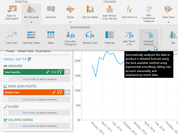
This option automatically applies the EXPSMOOTH function with default parameters so that your data is analyzed to find the best fitting forecast options, and then the optimal parameters are saved into the formula so that the result is calculated more efficiently next time.
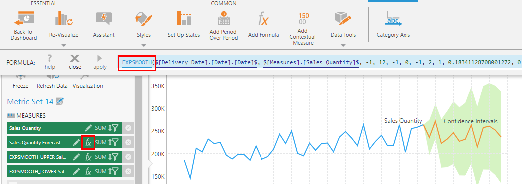
To see this, click the fx button on the new forecast measure in the Data Analysis Panel.
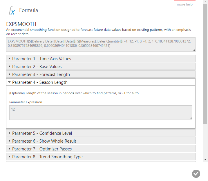
To read these parameters more easily, click the EXPSMOOTH function name to open the Formula dialog, then click to expand the section for each parameter to see its description and the current value.
6. Examples
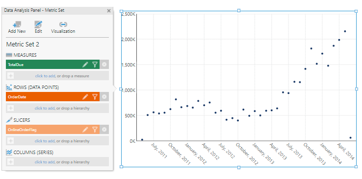
For the following examples of applying the exponential smoothing functions manually, first create a Point chart.
Add a measure (TotalDue), a time hierarchy (OrderDate), and a slicer (OnlineOrderFlag).
Edit the OrderDate hierarchy and change its Level to Month.
Filter the slicer to show only True values.
6.1. Single exponential smoothing
For some background information on single exponential smoothing, view this article from the National Institute of Standards and Technology.
With the chart selected on the canvas, go to the toolbar, click Data Tools, and then select Add Formula.
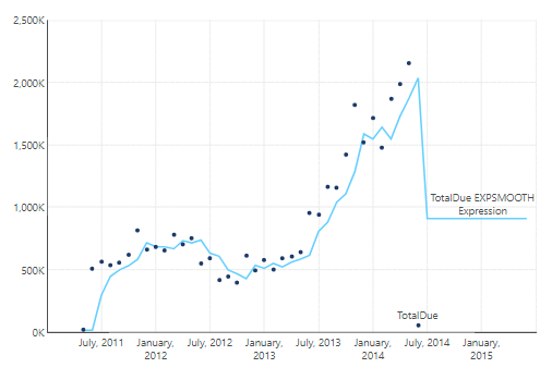
In the formula bar, click Visualization and select the line chart, then type the following and click apply:
EXPSMOOTH($OrderDate$, $TotalDue$, -1, -1, 0.95, 1, 10, 0, 0)

Here all the parameters are set to their default values, other than the following three:
- s3 is set to 1 to show the whole result
- s5 is set to 0, which means there is no trend smoothing
- s6 is set to 0, which means there is no season smoothing
The result is a forecasting extension of the Exponential Moving Average.
6.2. Double exponential smoothing
For some background information on double exponential smoothing, view this article from the National Institute of Standards and Technology.
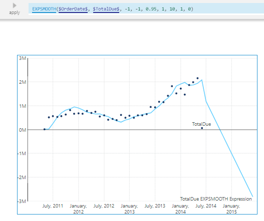
Open the Data Analysis Panel for the chart and edit the formula for the new measure.
Change the s5 parameter to 1, which will add additive trend smoothing to the single exponential smoothing result. Trend smoothing is an exponential moving average of the slope between points.
6.3. Triple exponential smoothing
For some background information on triple exponential smoothing, view this article from the National Institute of Standards and Technology.
Edit the formula again and change the s6 parameter to 1. This will add additive season smoothing to the double exponential smoothing result. Season smoothing is an exponential moving average of the values over repeating seasons.
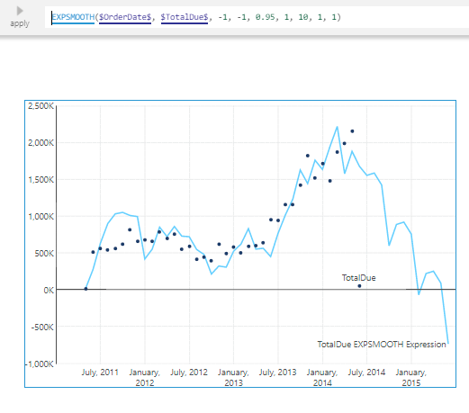
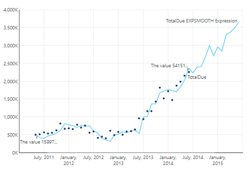
Notice that the first and last data points are very low and likely throw the forecasting off.
To correct that, switch to view mode, right-click the first data point and select Correct Value. Set the new value to 500000.
Similarly, correct the last data point to 2250000.
7. Notes
- The forecast will only go until the end of the time dimension or until the end of the OLAP time hierarchy.